One of the most important things for seagrass mapping with remote sensing is accuracy evaluation of classification. In general, accuracies of classification are evaluated with an error matrix (confusion matrix or contingency table) (Mumby and Green 2000). Accuracies are judged with a user accuracy, a producer accuracy, an overall accuracy and a tau coefficient (Ma and Redmond 1995).
1. Error Matrix (Pixels and percent)
The error is calculated by comparing the class of each ground truth pixel with the corresponding class in the classification image. Each column of the error matrix represents a ground truth class and the values in the column correspond to the classification image’s labeling of the ground truth pixels. Table 3 shows the class distribution in pixels and percentage for each ground truth class.
User accuracy is a measure indicating the probability that a pixel is Class A given that the classifier has labeled the image pixel into Class A. User accuracies are shown in the rows of the error matrix. For example, in Table 3, seagrass pixels obtained with a ground survey are 50 of which 39 and 11 are correctly and incorrectly classified, respectively. The percentages of the number of pixels correctly and incorrectly classified into the seagrass class were 78% and 22% (Table 3), respectively, corresponding to a user accuracy and an error of commission.
The producer accuracy is a measure indicating the probability that the classifier has labeled an image pixel into Class A given that the ground truth is Class A. For example, in Table 3, seagrass class of ground truth has a total of 48 pixels of which 39 and 9 pixels are correctly and incorrectly classified, respectively. The percentages of the number of seagrass pixels obtained with the ground survey classified correctly and incorrectly are 81.3% and 18.8% (Table 1), respectively, corresponding to a producer accuracy and an error of omission.
The overall accuracy is calculated by summing the number of pixels classified correctly and dividing by the total number of pixels. The pixels correctly classified are found along the diagonal of the error matrix table which lists the number of pixels that were classified into the correct ground truth class. The total number of pixels is the sum of all the pixels in all the ground truth classes. For example, in Table 3, the pixel counts of diagonal components consist of 39 pixels of seagrass and 51 pixels of sand, which are correctly classified pixels. The overall accuracy (81.8%) is obtained by dividing the correctly classified pixels number (39+51) by the total number of ground truth pixels (110).
Overall accuracy is the overall degree of agreement in the matrix. Generally, accuracies of classification of surface covers of coastal sea bottom are lower than those of land (e.g. Mumby et al, 1998). Mumby et al. (1999) stated that reasonable accuracy is between 60 and 80% for coarse descriptive resolution such as corals/seagrasses and mangroves/non-mangroves by using satellite images such as LANDSAT TM or pansharpened image of LANDSAT TM with SPOT. In any cases, overall accuracy is more than about 90% to monitor temporal changes in spatial distributions of bottom covers using a remote sensing (Mumby and Green, 2000).
2. Tau Coefficient
It is a reasonable way to describe the overall accuracy of a map but does not account for the component of accuracy resulting from chance alone. A chance component of accuracy exists because even a random assignment of pixels to habitat classes would include some correct assignments.
The Tau coefficient, T(e), is another measure of the accuracy of the classification to exclude a chance component and is expressed as the following equation:
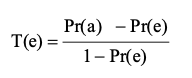
where Pr(a) and Pr(e) are the relative observed agreement among classes and hypothetical probability of chance agreement. For example, in Table 3, Pr(a) corresponds to the overall accuracy, 0.818. Pr(e) derived from two classes is 0.5. Then, we can obtain T(e) as 0.636 by dividing (0.818-0.50) with (1.0-0.5). The Tau coefficient ranges between -1.0 and 1.0. When the Tau coefficient is -1.0 and 1.0, classification is of perfect discrepancy and agreement, respectively. When the Tau is between 0.41 and 0.60, classification is of moderate agreement. When the Tau is between 0.61 and 0.80, classification is of good agreement. When the tau is over 0.80, classification is of nearly prefect agreement.
The variance of Tau, σ2, is calculated as the following equation (Ma and Redmond 1995):
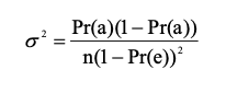
where n is the number of samples. Confidence intervals are then calculated for each Tau coefficient at the 95% confidence level (1-α), using the following form:
![]()
where Z is a standard normal distribution with the lower bound of α/2. Using Table 3, we obtain 95%CI as 0.636 ±0.001. The coefficient’s distribution approximates to normality and Z-tests can be performed to examine differences between matrices (Ma and Redmond 1995). When two different classification methods (method 1 and method2) are applied, Z-tests are conducted to verify whether significant difference in Tau coefficients (T1 and T2) between results obtained by method 1 and method 2 exists or not using the following equations:
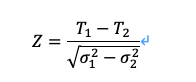
where σ2 is the variance of the Tau coefficient, calculated from equation (10). We can examine whether Tau coefficients have a 95% probability of being different or not.